
model quantization
what is it and common use cases

I came across model quantization while on a walk with one of my coworkers and immediately started rabbit holing. I’m here to share my rabbit hole.
what is quantization?
In the world of machine learning (ML), there's an ongoing quest for models that can make accurate predictions while being fast and efficient. There are many many methods being explored from model distillation to pruning, etc. One powerful technique that addresses this challenge, in my opinion in the most interesting way, is model quantization. If you’ve ever had to squeeze a large amount of data into a small space—like compressing a long essay into a few bullet points—you can think of quantization as a similar process.
leading with an analogy
Imagine you’re trying to move a heavy suitcase from point A to point B. Now, let’s say that suitcase represents a machine learning model, and inside it are tons of weights—numbers that help the model make predictions. But this suitcase is huge, and moving it takes time and resources. Model quantization is like compressing that suitcase, making it lighter and smaller while keeping the contents intact (or close to intact).
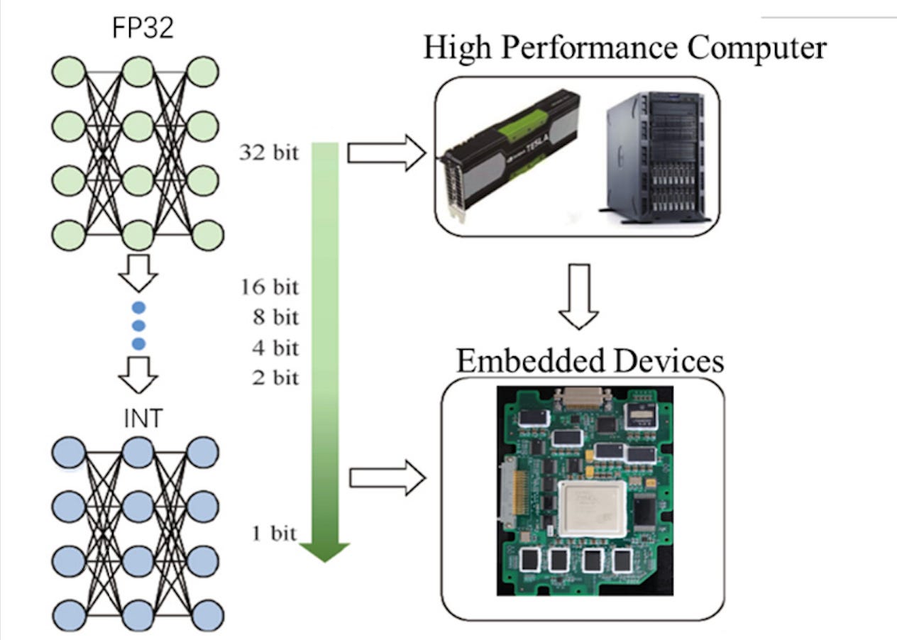
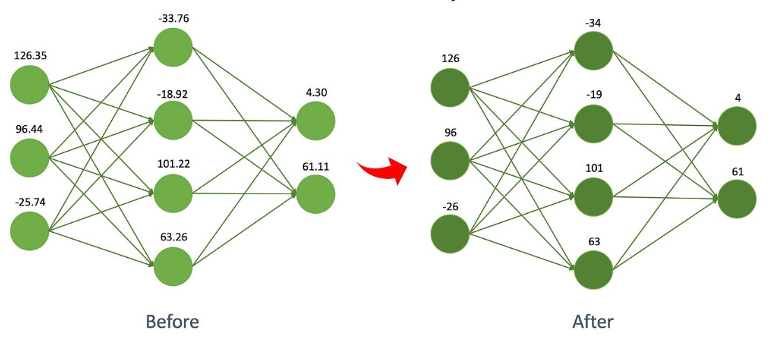
There are many different approaches for how they can be done, but the most common way, and what I’ve been investigating is by reducing the precision of the model's weights from high-precision floating-point numbers (like 32-bit floats) to smaller, more compact integers (like 8-bit integers). This makes the model more efficient, with smaller memory requirements and faster computation. All the research I’ve been doing has been working on embedded systems so this compression is the only way to actually train models in these very limited spaces.
You’re probably wondering why we convert from 32 bits to 8 bits. Without going too deep into how CPUs work just know that when working with floating-point numbers (often 32-bit or 64-bit), we’re dealing with a representation that’s much more complex than the traditional 8-bit integers, and this complexity introduces a need for more computational power. Floating-point numbers are like very detailed, high-resolution pictures. They store both the magnitude (how big the number is) and the precision (the level of detail of the number), which allows them to represent a wide range of values, including very small and very large ones, as well as fractions.
In contrast, 8-bit integers are much simpler. They can only represent whole numbers between -128 and 127. There’s no need to worry about magnitude or precision in the same way—just the value itself.
Since 8-bit integers don’t have to store as much information and don't require complex handling for decimal points or exponents, operations involving them are much quicker and require less computational power.
The flavour of Quantization
There are many different approaches to quantization, I’ll attempt to highlight a few. Some of the most interesting approaches I’ve seen applied have been from people who use a mix of these ideas.
Post-Training Quantization (PTQ)
Imagine you've painted a beautiful picture, and you’re ready to hang it up in a small frame. You could shrink the painting to fit the frame, but it wouldn’t alter the essence of the artwork itself. This is similar to Post-Training Quantization (PTQ). In PTQ, you first train a model using high-precision numbers. Once the training is done, you take that pre-trained model and apply quantization, which reduces the precision of the weights, usually to 8-bit integers.
The beauty of PTQ is that it's fast. Since you’re not retraining the model from scratch, it’s like a shortcut to a lighter model that’s ready to be deployed. However, because you’re simplifying the model’s weights, it can sometimes lead to a slight drop in accuracy—especially for complex models that rely on higher precision to make fine-tuned predictions. PTQ is a great option when you’ve already trained a model and just need to compress it for deployment in resource-constrained environments like mobile devices or embedded systems.
Quantization-Aware Training (QAT)
Now, instead of shrinking the painting after it’s completed, you start the painting process with the knowledge that it’s going to be framed smaller. This is what Quantization-Aware Training (QAT) does. Rather than applying quantization after training, QAT builds quantization into the process itself from the beginning.
The process works like this: you first train the model using full-precision numbers, just like normal. But during training, you simulate quantization meaning that, even though the model is still learning, the weights are treated as if they’re low precision (like 8-bit numbers). This helps the model adjust, so when it's time to deploy, it already "knows" how to work with lower precision weights.
The key benefit of QAT is that because the model is trained with quantization in mind, it’s usually more robust to the changes that happen when you compress it. As a result, QAT often leads to better accuracy after quantization compared to Post-Training Quantization. If you're building a model from scratch and aiming for deployment in a low latency, resource constrained environment, QAT is a great choice.
Fine Tuning After Post Training Quantization
Sometimes, the first pass at quantization doesn’t go as smoothly as you’d like. It’s like resizing a picture and realizing that a bit of the detail got lost in the process. In this case, Fine Tuning After Post Training Quantization (also known as PTQ + Fine-tuning) offers a solution.
First, you apply post-training quantization to a pre-trained model, just like we discussed earlier. The model gets compressed, but you notice some accuracy loss. To recover some of that lost accuracy, you do a bit of retraining, or "fine tuning," on the quantized model. This retraining typically involves a smaller learning rate, which means you’re making small adjustments to the model to help it adapt to the new, compressed weights.
This method works well when PTQ leads to noticeable accuracy drops, and you need to tweak the model just a bit to bring it back in line. It’s a helpful middle ground between the speed of PTQ and the accuracy benefits of QAT, especially when you’ve already applied quantization and need to fine-tune for better performance.
Once you’ve decided on the right approach for quantizing your model, the next step is converting the numbers themselves into a more compact form, typically reducing them to 8 bits or fewer. This is where we explore two main strategies for converting the values: symmetric quantization and asymmetric quantization, both of which come with their own strengths and nuances.
Symmetric Quantization
Think of symmetric quantization as balancing a seesaw with a heavy rock at both ends. The range of values in the model is centred around zero, meaning both negative and positive numbers are treated equally, almost like two equal forces pulling on each side of the seesaw.
In practice, both positive and negative values are mapped to the same scale. The zero point often sits right in the middle, and the number range is split into evenly spaced intervals. For example, with 8-bit symmetric quantization, you might have values that range from -128 to 127, with zero right at the centre. Although there are many drawbacks to this, it is greatly skewed by outliers, there is often empty space on either side of the zero because you’re forcing it to be the centre of the data which in most cases isn’t accurate.
Asymmetric Quantization
Now, picture asymmetric quantization as a seesaw that’s tilted to one side. Unlike symmetric quantization, the range here doesn’t revolve around zero. Instead, each side of the seesaw gets a different treatment, with the scale being adjusted independently for positive and negative values.
In this approach, the zero point can be anywhere along the range, not necessarily at the center. For instance, with 8-bit asymmetric quantization, your values might range from 0 to 255, or they might range from -127 to +128, with a zero-point offset. This requires calculating a specific zero-point offset to adjust the scaling, allowing the positive and negative values to have different ranges.
Clustering-based Quantization
Let’s step into a more advanced technique: clustering-based quantization, which is like grouping similar colours in a painting and using one colour to represent all of them, rather than trying to represent each colour individually. This method is about finding patterns and grouping similar things together to simplify the overall representation.
Here’s how it works: First, a clustering algorithm (like k-means) is applied to the model's weights. The idea is to identify groups of weights that are close to each other in value. Once the clusters are identified, each cluster is represented by a single "centroid" (which is just the average of the group). All the weights in that cluster are then mapped to the centroid value.
A lot of the most interesting implementations I’ve seen flip-flop and have the inputs use either asymmetric or symmetric and the weights use the opposite.
Model quantization is a powerful tool in the machine learning toolbox. It helps make large, complex models more efficient and accessible, especially in environments with limited resources. Whether it’s making edge devices smarter or improving real-time applications, quantization is the key to making AI more practical and widespread.
So next time you’re working with a large model, remember: it might just need a little quantization to make it work wonders. It’s all about finding the balance between size, speed, and accuracy—and with the right technique, you can have the best of all worlds.
Also if you’re curious about how these implementations, I’ll provide the source code from tensorflow. Also as a side note, if you want to play around with this yourself different hardware has its own apis/implementation of calling your script so it’s actually very easy to build on your own.
https://github.com/tensorflow/tensorflow/tree/master/tensorflow/compiler/mlir/quantization
enjoy